Time of Flight

Compute the time of flight from the inlet/outlet. The underlying workhorse uses the marching_map() function from PoreSpy.

---

Import packages

import dpm_tools as dpm
import porespy as ps
import numpy as np
import matplotlib.pyplot as plt

[15:58:59] ERROR    PARDISO solver not installed, run `pip install pypardiso`. Otherwise,          _workspace.py:56
                    simulations will be slow. Apple M chips not supported.                                         

Demonstration image

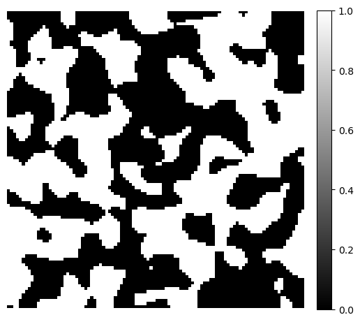
To demonstrate the distance transforms, we generate a simple 3D binary image using the PoreSpy blobs generator function. The example image size is \(100 \times 100 \times 100\).

image = ps.generators.blobs(shape=[100, 100, 100])

fig, ax = plt.subplots(figsize=[6, 6])
im = ax.imshow(image[1], cmap="binary_r")
fig.colorbar(im, fraction=0.046, pad=0.04)
ax.axis(False)

(-0.5, 99.5, 99.5, -0.5)

Time of Flight

The time of flight (ToF) is computed as the solution to the Eikonal equation,

\[ |\nabla T(x)| = \frac{1}{|v(x)|}, \]

where \(T(x)\) is the time of flight to point \(x\) and \(v(x)\) is the stead-state velocity field.

The equation describes a wavefront moving with speed \(|v(x)|\) and results in the first arrival time of the front to location \(x\). For pore scale characterization, the ToF map helps to visualize flow paths and quantify connectivity and tortuosity. Numerically, the solution is obtained using the Fast Marching Method.

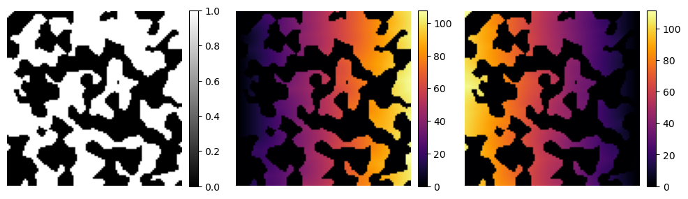
The tof function in the dpm_tools.metrics module expects a 2D or 3D np.ndarray where the phase of interest (foreground) is labeled as 1. The function computes the time of flight from the left or right faces (denoted by ‘l’ or ‘r’). It also “detrends” the result by default, meaning it subtracts away the underlying solution assuming no solid matrix is present in the image.

image_tofl = dpm.metrics.time_of_flight(image, 'l', detrend=False)
image_tofr = dpm.metrics.time_of_flight(image, 'r', detrend=False)

fig, ax = plt.subplots(1, 3, figsize=[12, 6])

im = ax[0].imshow(image[50], cmap="binary_r")
fig.colorbar(im, fraction=0.046, pad=0.04)
ax[0].axis(False)

im = ax[1].imshow(image_tofl[50], cmap="inferno")
fig.colorbar(im, fraction=0.046, pad=0.04)
ax[1].axis(False)

im = ax[2].imshow(image_tofr[50], cmap="inferno")
fig.colorbar(im, fraction=0.046, pad=0.04)
ax[2].axis(False)

(-0.5, 99.5, 99.5, -0.5)