LBPM Simulation
This guide provides step-by-step instructions for running Lattice Boltzmann for Porous Media (LBPM) on the Digital Porous Media Portal (DPMP) for:
- Single-phase (MRT) permeability simulations on x86 CPUs
- Single-phase (MRT) permeability simulations on GPUs
- Morphological drainage simulations on GPUs
- Multiphase (Color) simulations on GPUs
Launch the Application
-
Log in to the DPMP and navigate to the
My Dashboardinterface.
-
Navigate to the
Applicationstab in the left-hand menu (1). Then, navigate to theSimulationcategory (2). Click on the simulation tool you want (e.g.,LBPM MRT CPU (Lonestar6)) from the list of available simulation applications (3).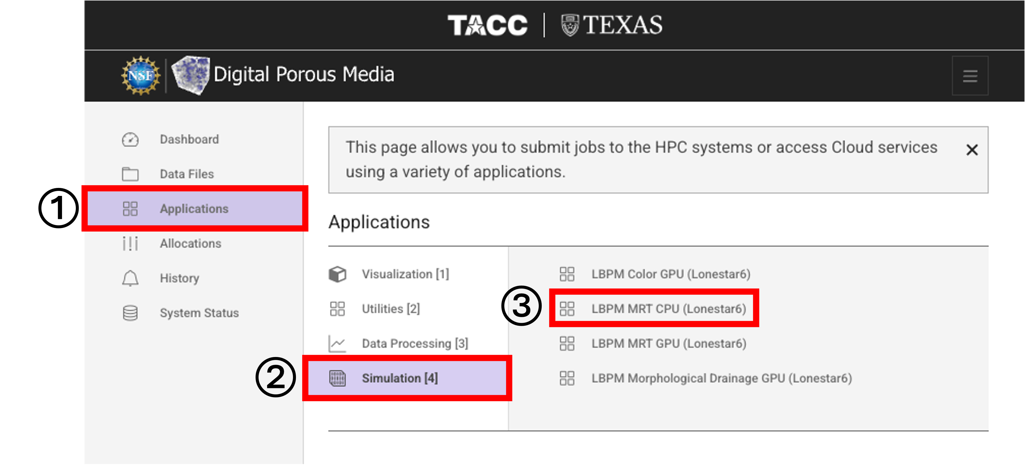
Inputs
-
Under
Inputs, clickSelectnext toInput Fileto browse for the input database (.db) file for the LBPM simulation. Here, a pore of Berea sandstone (a.k.a. the Chicken pore) is used as an example.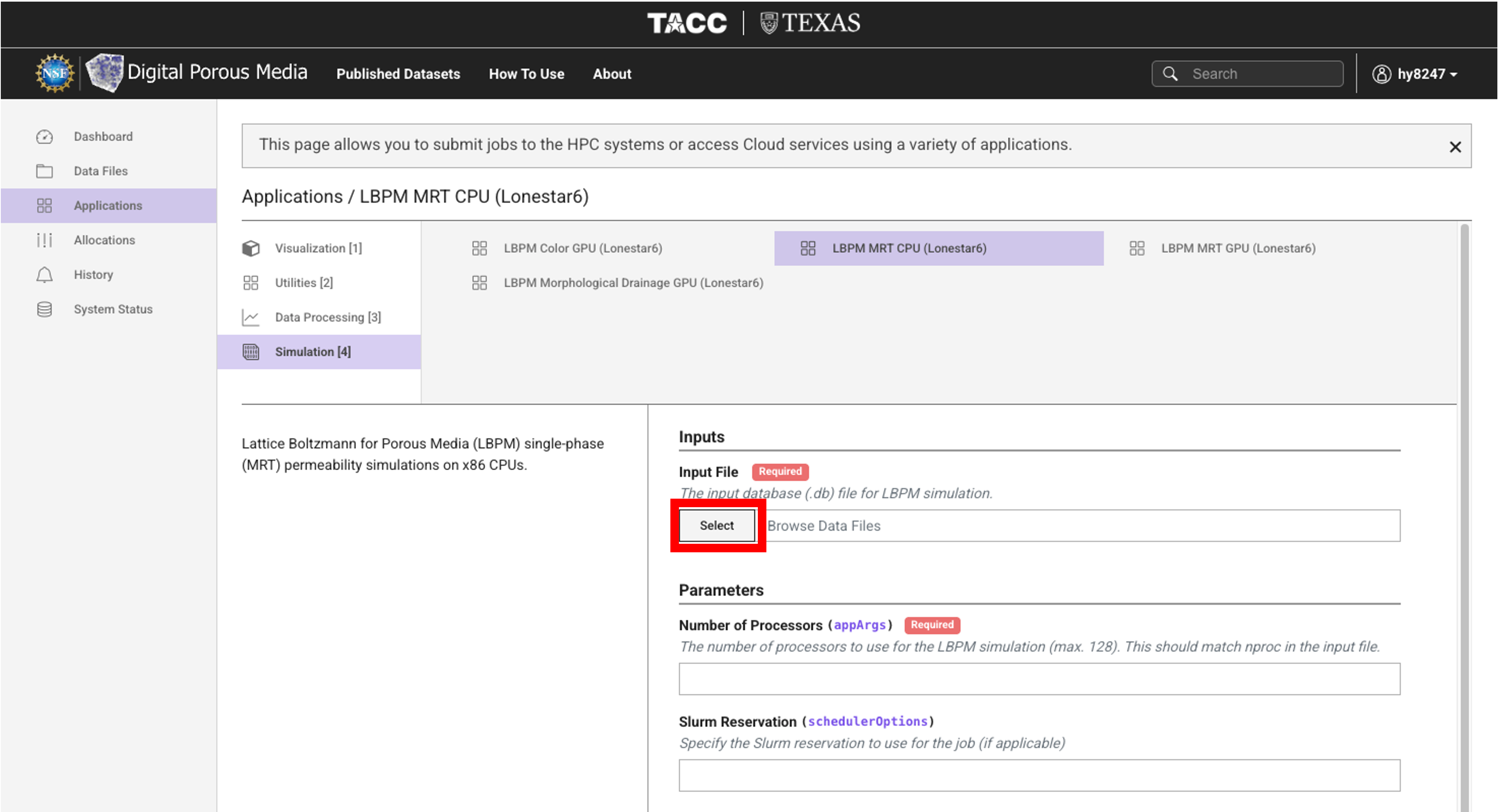
-
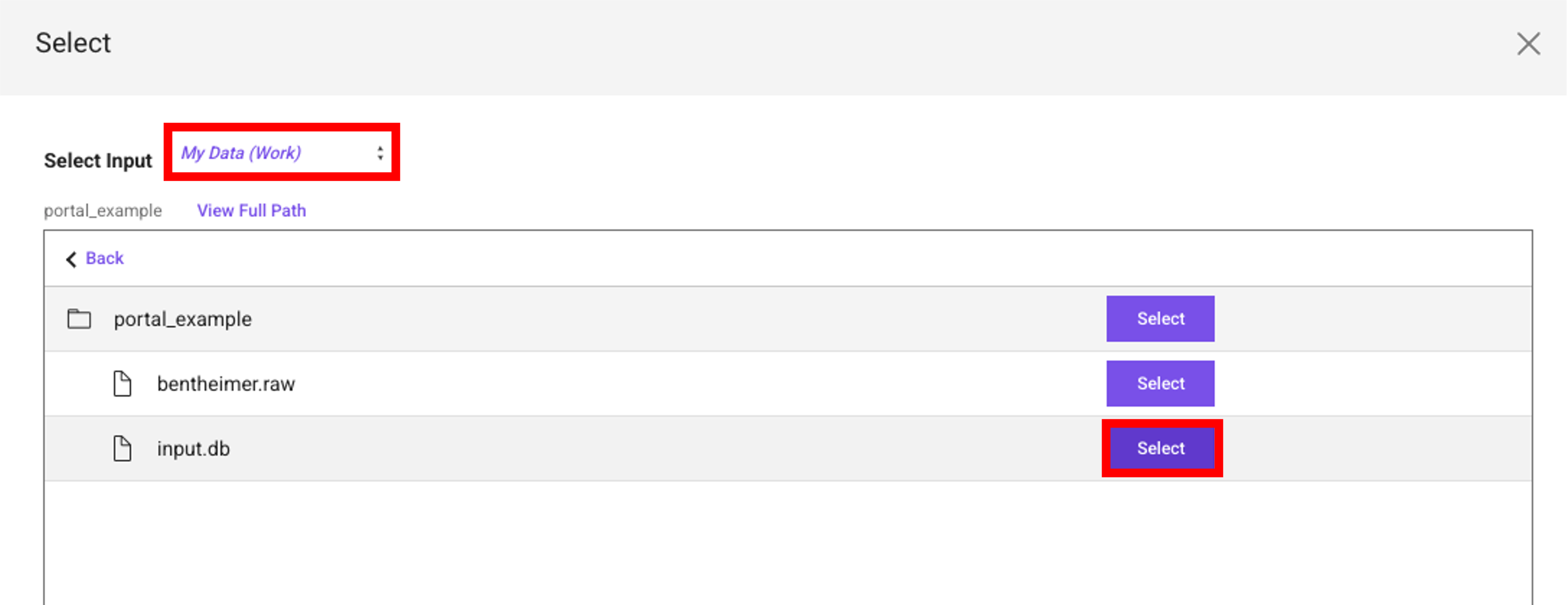
Navigate to the file location and select the input file.
-
Use the appropriate input file for each type of simulation.
Single-phase (MRT) permeability simulations on x86 CPUs
Below is an example
input.dbfile for a single-phase (MRT) LBPM simulation. In this example,nprocis set to1, 1, 1, for a total of 1 processor.Domain { Filename = "berea_pore_110.raw" ReadType = "8bit" nproc = 1, 1, 1 n = 110, 110, 110 N = 110, 110, 110 voxel_length = 1 ReadValues = 1, 0 WriteValues = 0, 2 BC = 0 } MRT { tau = 0.7 F = 0.0, 0.0, 1.0e-5 timestepMax = 1000000 tolerance = 0.0001 }Morphological drainage simulations
Below is an example
input.dbfile for a morphological drainage LBPM simulation. In this example,nprocis set to1, 1, 1, for a total of 1 processor.Domain { Filename = "berea_pore_110.raw" ReadType = "8bit" nproc = 1, 1, 1 n = 110, 110, 110 N = 110, 110, 110 voxel_length = 1 ReadValues = 1, 0 WriteValues = 0, 2 BC = 0 Sw = 0.10 }Multiphase (Color) simulations
Below is an example
input.dbfile for a color LBPM simulation. In this example,nprocis set to1, 1, 3, for a total of 3 processors.Domain { Filename = "berea_pore_110.raw" ReadType = "8bit" nproc = 1, 1, 1 n = 110, 110, 110 N = 110, 110, 110 voxel_length = 1 ReadValues = 1, 0 WriteValues = 0, 2 BC = 0 Sw = 0.10 } MRT { tau = 0.7 F = 0.0, 0.0, 1.0e-5 timestepMax = 1000000 tolerance = 0.0001 } Color { protocol = "fractional flow" capillary_number = 1e-3 tauA = 0.7 // relaxation time for fluid A (labeled as "1") tauB = 0.7 // relaxation time for fluid B (labeled as "2") rhoA = 1.0 // density for fluid A (in lattice units) rhoB = 1.0 // density for fluid B (in lattice units) alpha = 5e-3 // controls the surface tension beta = 0.95 // controls the interface width F = 0, 0, 1e-4 // controls the external force Restart = false // initialize simulation from restart file? timestepMax = 10000000 // maximum number of timesteps to perform before exit ComponentLabels = 0 // number of immobile component labels in the input image ComponentAffinity = 1.0 // wetting condition for each immobile component WettingConvention = "SCAL" } Analysis { analysis_interval = 10000 // Frequency to perform analysis visualization_interval = 10000 // Frequency to write visualization data restart_interval = 1000000 // Frequency to write restart data restart_file = "Restart" // Filename to use for restart file (will append rank) N_threads = 3 // Number of threads to use for analysis load_balance = "default" // Load balance method to use: "none", "default", "independent" } Visualization { format = "hdf5" write_silo = true // write SILO databases with assigned variables save_8bit_raw = true // write labeled 8-bit binary files with phase assignments save_phase_field = true // save phase field within SILO database save_pressure = true // save pressure field within SILO database save_velocity = true // save velocity field within SILO database } FlowAdaptor { fractional_flow_increment = 0.05 endpoint_threshold = 0.1 skip_timesteps = 10000 min_steady_timesteps = 50000 max_steady_timesteps = 500000 }Note
A detailed description and example input files of simulations can be found in the LBPM Documentation.
Parameters
CPU
Enter the Number of Processors for the LBPM simulation. This value must match nproc in the selected input.db file.
-
In this example,
nproc = 1, 1, 1, so the number of processors is1.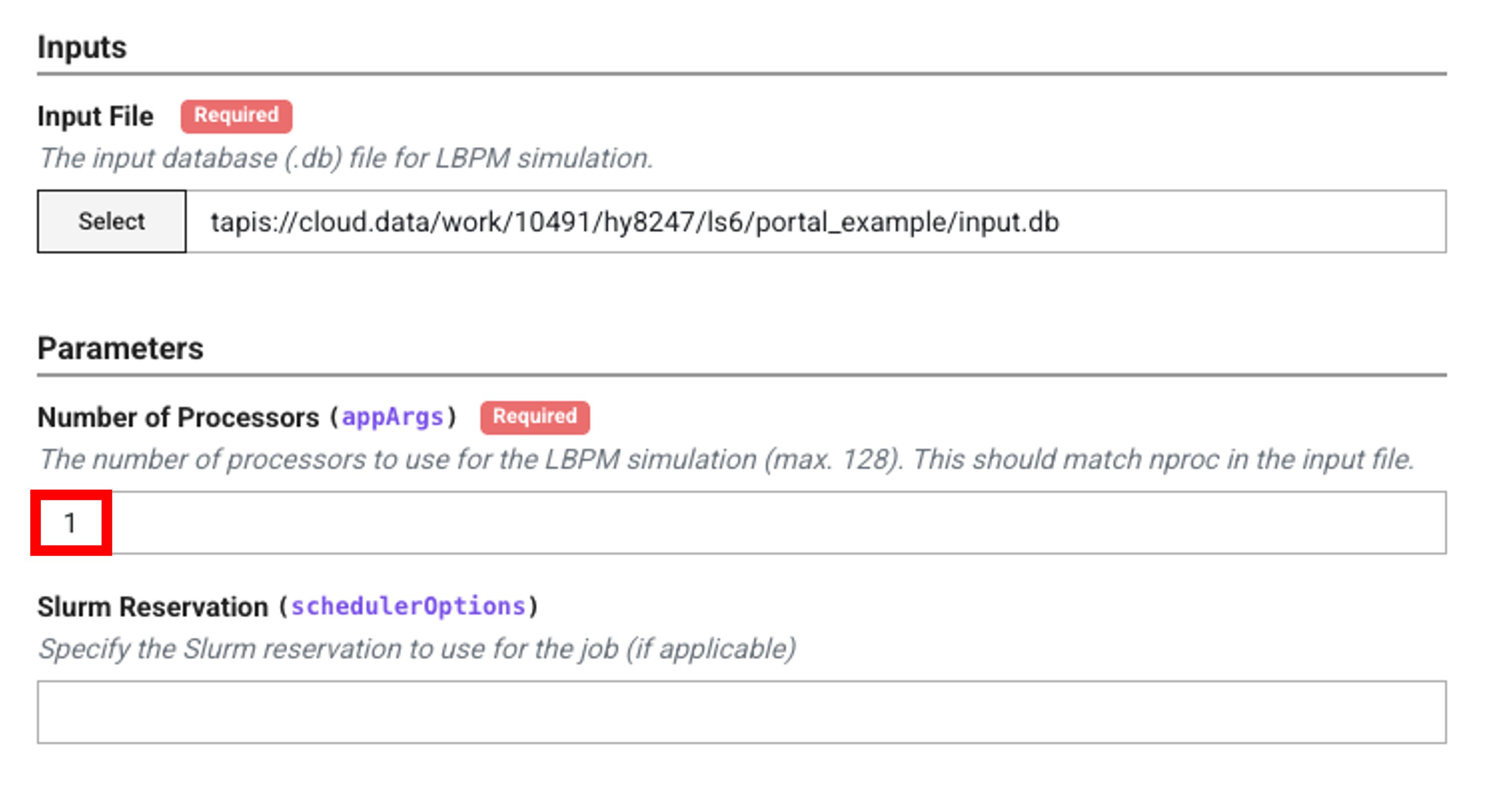
Note
The number of processors cannot exceed 128.
GPU
Enter the Number of GPUs for the LBPM simulation. This value must match nproc in the selected input.db file.
-
In this example,
nproc = 1, 1, 3, so the number of processors is3.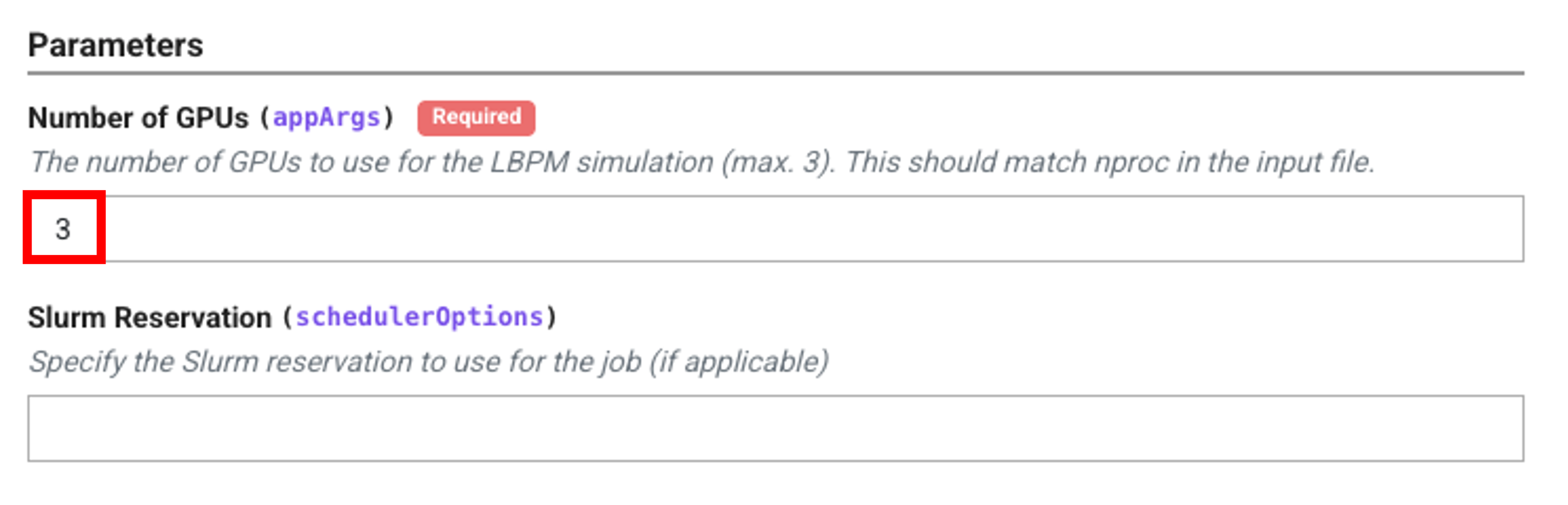
Note
The number of GPUs cannot exceed 3.
Configuration
-
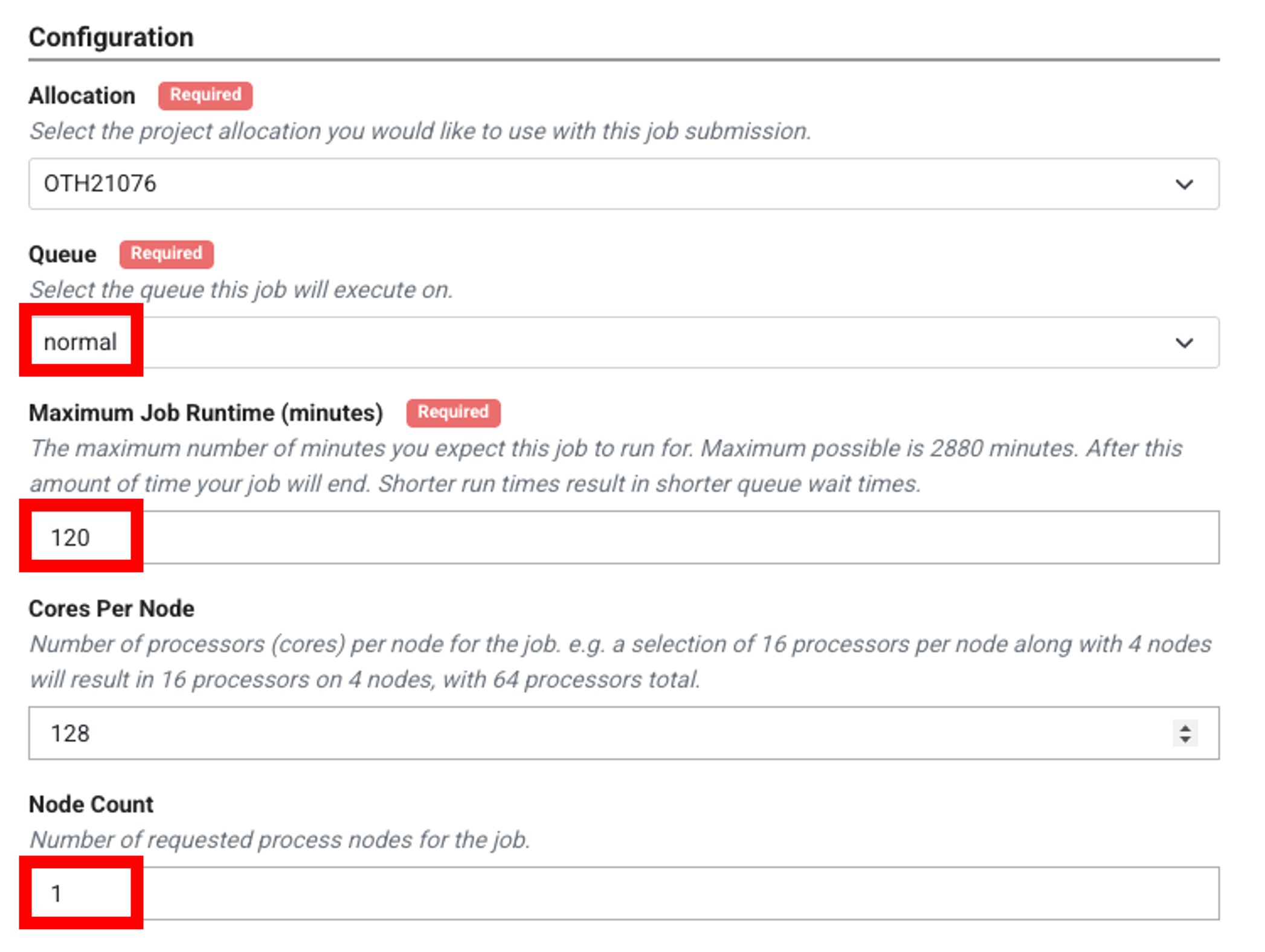
Select the
Allocationto be used for this job submission, then select theQueueon which this job will execute.- For CPU, available queues include
normal,vm-small, etc. - For GPU, available queues include
gpu-a100-small,gpu-a100,gpu-h100, etc. - A detailed description of available queues on Lonestar6 can be found in the TACC Lonestar6 documentation.
-
The current status of queues on Lonestar6 (idle nodes, running jobs, and waiting jobs) can be found under
System Status > Lonestar6.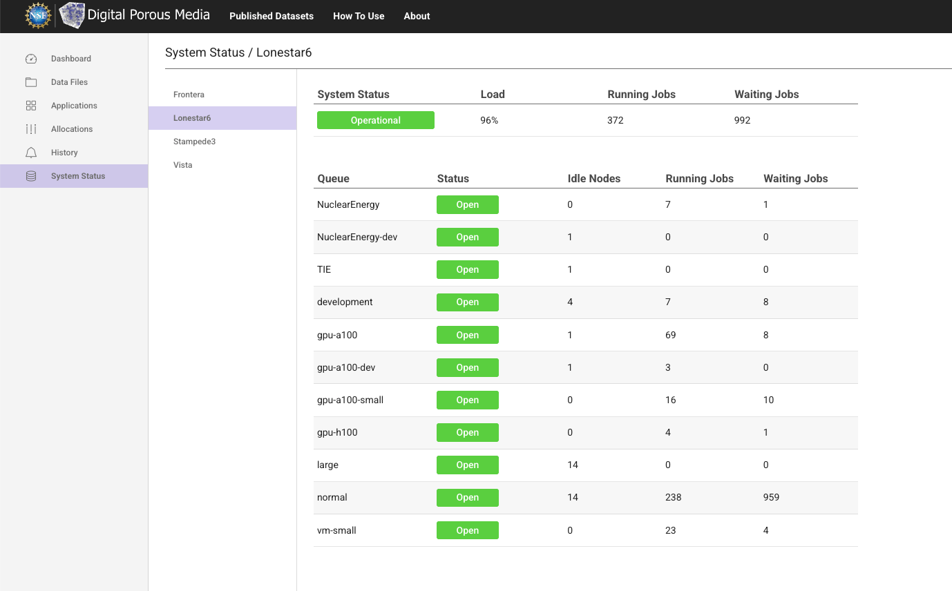
- For CPU, available queues include
-
Set the
Maximum Job Runtime,Cores Per Node, andNode Countfor the job. In most cases, aNode Countof 1 is recommended.
Outputs
-
Enter a
Job Name, and specify theArchive SystemandArchive Directorywhere output files will be stored after the job completes. ClickSubmit.-
The default
Archive System,cloud.data, points to the$WORKfile system on Lonestar6. The defaultArchive Directorycreates a folder namedtapis-jobs-archiveunder the user's$WORKdirectory, where output files can be found after the job completes. -
To archive outputs to a different location within
$WORK, provide the absolute path to the desired directory, for example/work/<useridentifier>/<username>/ls6/my_output_folder, in place of the default. -
To archive outputs to
$SCRATCHinstead, set theArchive Systemtols6and provide the absolute path to the desired directory on the$SCRATCHfile system.
Output Directory Archive System Archive Directory Default cloud.data/work/<useridentifier>/tapis-jobs-archive/${JobCreateDate}/${JobName}-${JobUUID}Work folder cloud.datapath to directory in $WORKfolder (ex:/work/<useridentifier>/<username>/ls6/my_output_folder)Scratch folder ls6path to directory in $SCRATCHfolder (ex:/scratch/<useridentifier>/<username>/my_output_folder)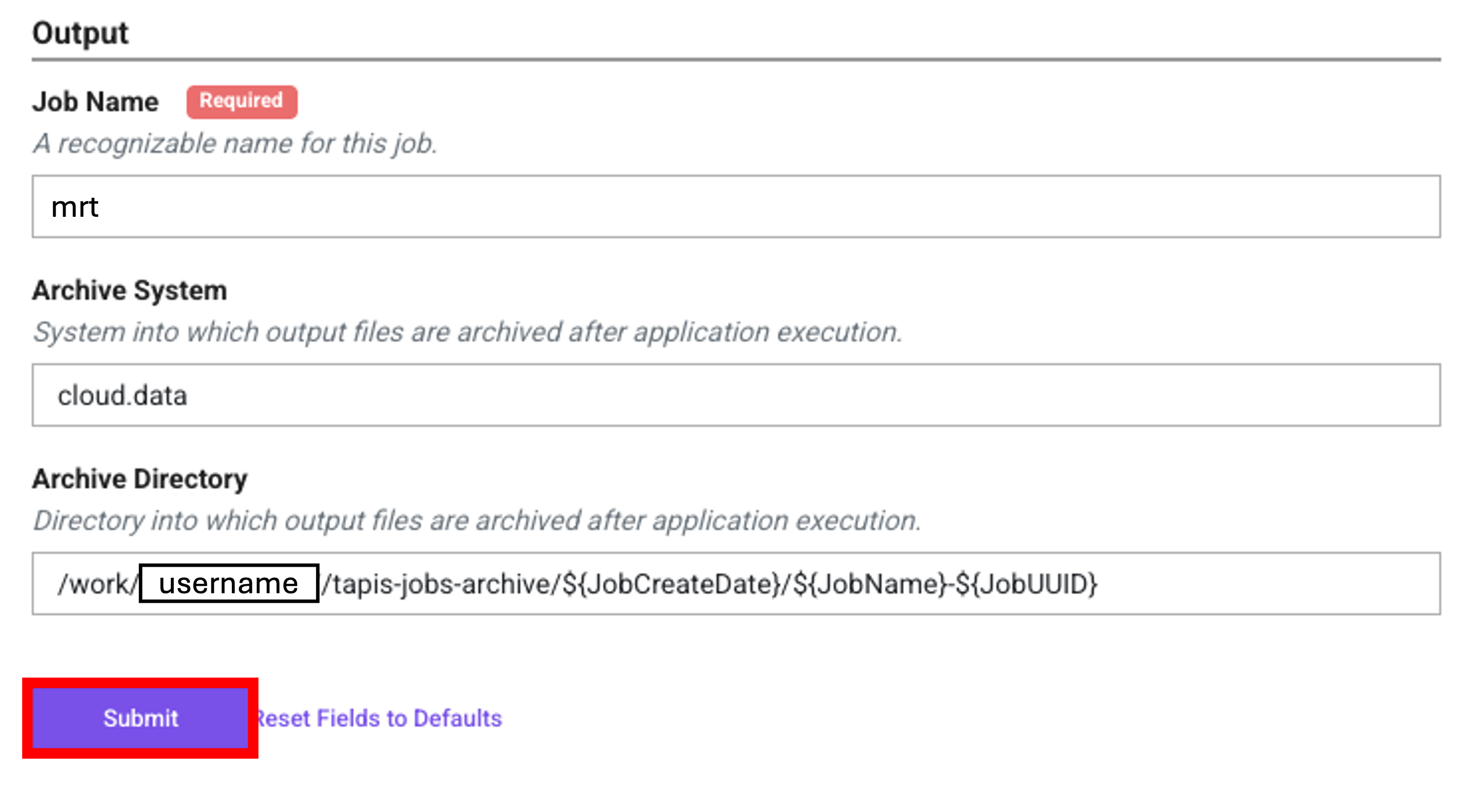
-
-
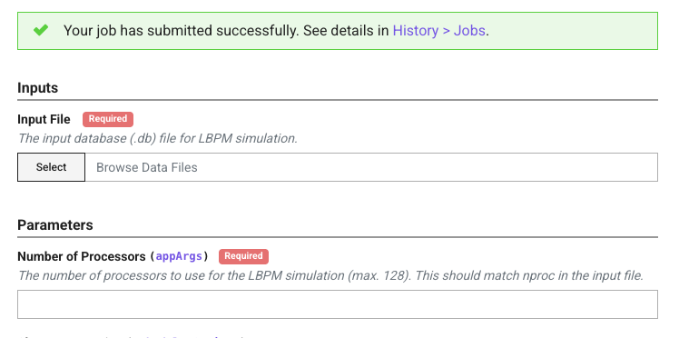
Once submitted, a confirmation message will be displayed.
Monitor and Retrieve Results
-
Navigate to
History > Jobs, locate the job byJob Name, and clickView Details.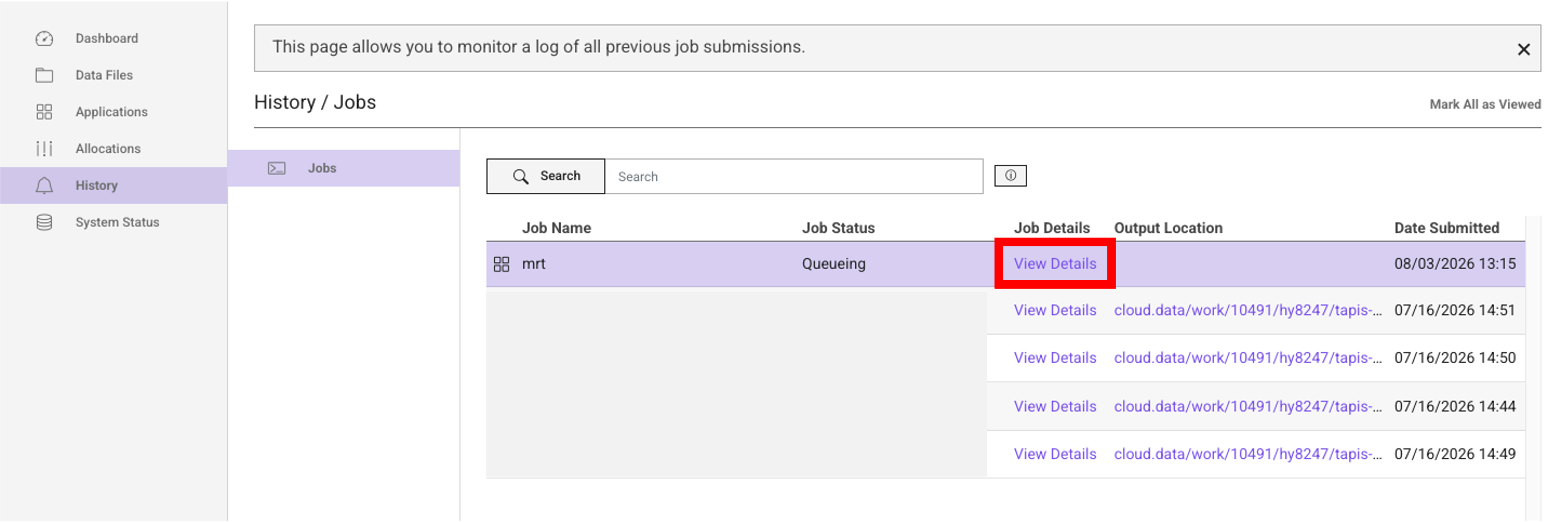
-
In the job details panel, click
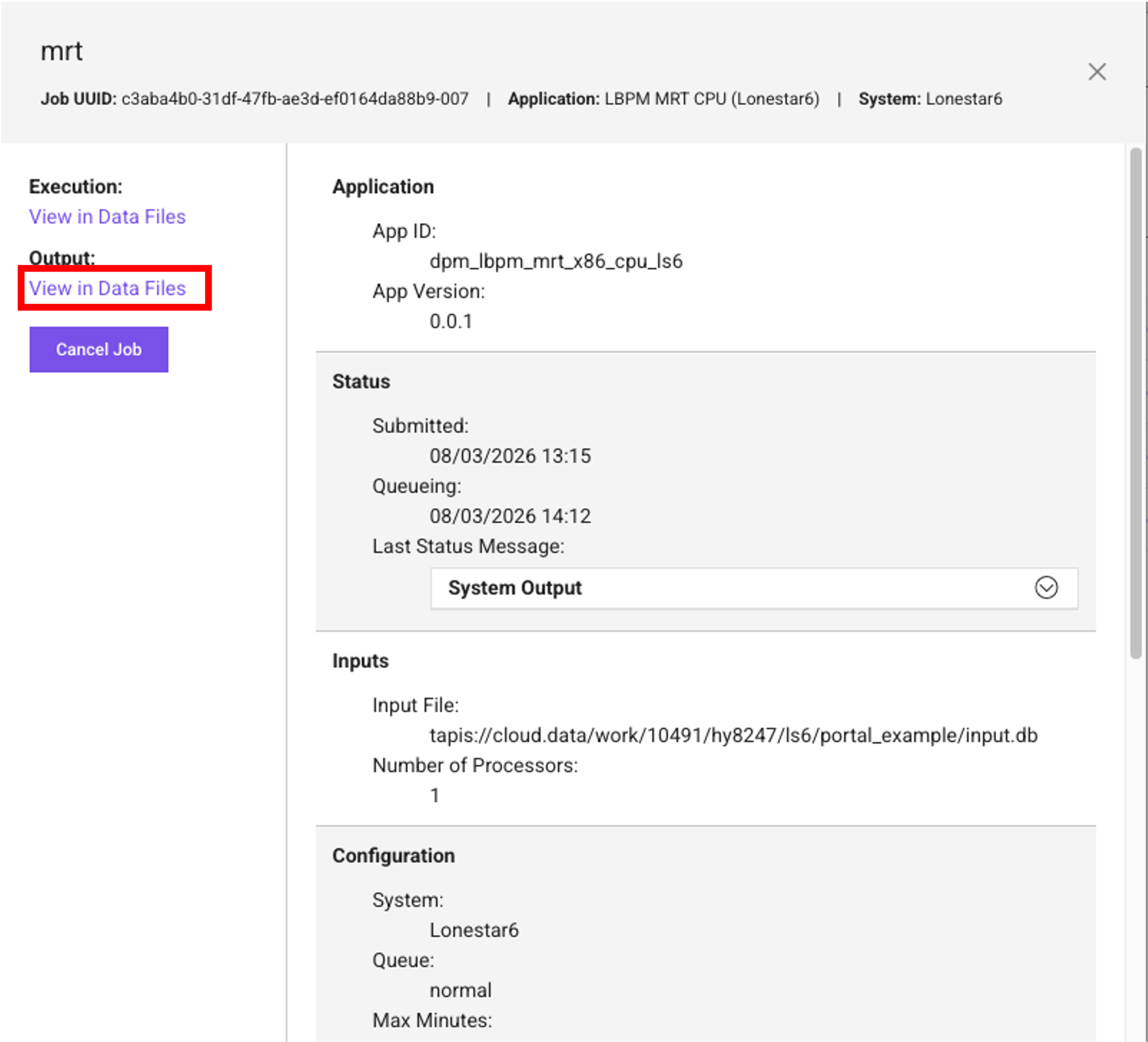
View in Data FilesunderOutputto access the output files.